Modeling Barium-137m Radioactive Decay
Geiger-counter decay curve, chi-squared validation, and Poisson vs. Gaussian count statistics
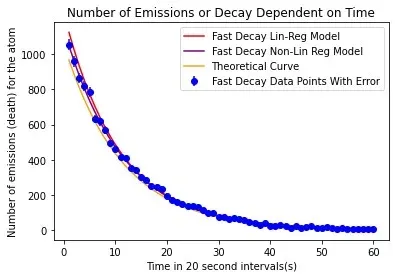
An exponential (non-linear) decay model fit the Barium-137m emission data with a reduced chi-squared of 0.8, against 1.1 for the linear fit, and its residuals sat near zero across all 60 time intervals.
Result
The exponential decay model fit the Barium-137m data with a reduced chi-squared of 0.8, beating the linear fit’s 1.1, and its residuals stayed near zero across all 60 intervals. The goal was straightforward: measure Ba-137m emissions over time with a Geiger counter, then settle which regression model actually describes radioactive decay. A second goal was to characterize the random nature of the counts themselves using Poisson and Gaussian statistics.
Approach
A Ba-137m source was eluted and counted on a Geiger counter in 20-second intervals out to 60 intervals. Background radiation was measured separately and subtracted from every sample, and each count’s uncertainty was propagated as the square root of the count plus the mean background (u = sqrt(N + B)), which is the right error model for Poisson-distributed counts.
Two models were fit to the background-subtracted counts in Python using SciPy’s curve_fit: a linear regression on the natural log of the counts, and a direct non-linear fit of the exponential y = bexp(-at). Both were compared against a theoretical curve built from Ba-137m’s known 2.6-minute half-life. Fit quality was judged with reduced chi-squared and with residual plots, not by eye.
Findings
The residual plots told the cleanest story. The linear model left a large, structured residual that decayed with time, a sign it was the wrong shape, while the exponential model’s residuals scattered tightly around zero. Reduced chi-squared agreed: 0.8 for the exponential fit versus 1.1 for the linear one.
The half-life estimates were less decisive. The linear fit gave 3.57 minutes (plus or minus 1.41) and the non-linear fit gave 3.75 minutes (plus or minus 0.944), both above the 2.6-minute reference. That gap, and the sub-one chi-squared, both point at the same limitation: too few samples. For the slow-decay counts, the Poisson and Gaussian distributions were nearly identical around a mean near 110, exactly as Poisson statistics predict at a high mean.
Why it matters
This is a worked example of letting the statistics, not intuition, choose the model. The residual analysis and chi-squared comparison make the exponential fit’s superiority defensible, and the honest read on the half-life discrepancy (more samples needed) is the kind of conclusion that holds up.